Audioscan Speechmap® Audibility Mapping
Speechmap® is a trademarked audibility mapping system introduced by Audioscan in 1992. It was inspired by the work of Margo Skinner and David Pascoe at Central Institute for the Deaf (CID) who developed a fitting method based on amplifying a calibrated real speech signal to the approximate center of the auditory area. Speechmap® was the first embodiment of this concept ever in a commercial system. It used simulated speech signals to create a map of the amplified speech region within the residual auditory area – hence the name “Speechmap”. Studies by Stelmachowicz et al (1996) and Scollie et al (2002) provided proof that the simulated speech signals used in Speechmap were good predictors of real speech output for compression hearing aids of the time.
In 2001, the Audioscan Verifit® introduced calibrated real speech signals to Speechmap and was the first system employing such signals. Audioscan has been the leading innovator in the use of speech and speech-like signals for hearing instrument fitting and has an unparalleled understanding of the science behind these methods. This unique expertise is what makes Speechmap different from other similarly-named audibility mapping systems.
Audioscan Speechmap: Key Features
1) Provides a variety of digitally-recorded real-speech signals as well as allowing the use of live speech.
Why it matters: The use of recorded speech material ensures repeatable measurements. Recorded speech is the gold standard signal (vs. noise or tonal signals) that allows for testing without negative interaction with adaptive features and therefore does not require use of a ‘verification mode’ where adaptive features are turned off .
2) The speech signals are controlled in real time to produce a calibrated, controlled spectrum in the sound field as well as in the test box
Why it matters: Fitting methods such as DSL, NAL-NL1, NAL-NL2, and the Speech Intelligibility Index (SII) all assume specific spectra for speech at various vocal efforts. If these specified spectra are not delivered to the hearing aid when matching these fitting targets or when calculating the SII, significant errors will result.
3) All amplified speech passages, both recorded and live, are analyzed in 1/3 octave bands over several seconds to provide the long-term average speech spectrum (LTASS).
Why it matters: Fitting targets for DSL, NAL-NL1, NAL-NL2, and the SII calculation all assume an LTASS obtained by averaging 1/3 octaves bands of speech over
several seconds. When broadband signals are analyzed in narrow bands to produce a spectrum, the SPL in each band depends on the width of the band.
For example, the spectrum of a speech signal will appear nearly 10 dB lower on systems which use 1/24 octave analysis bands rather than the 1/3 octave analysis used in Speechmap. When fluctuating signals are analyzed, the averaging time used to compute the SPL in each band influences the result. An accurate LTASS can only be obtained using averaging times of 10 seconds or more. Matching targets or calculating the SII using curves obtained using bands other than 1/3 octave or analysis times shorter than 10 seconds will result in errors in the SII and in the fitting.
4) The amplified speech region (speech banana) is calculated from the statistical properties of the measured speech using an integration time similar to that of the ear.
Why it matters: The range between speech valleys and speech peaks (speech region) is often depicted as extending from 18 dB below the LTASS to 12 dB above. However, this depends on the talker and on the operation of the compression system in the hearing instrument. Rather than just drawing the speech region as a 30 dB range above the LTASS, Speechmap audibility mapping shows the top of the speech region as the SPL exceeded 1% of the time (the 99th percentile) and the bottom of the speech region as the SPL exceeded 70% of the time (30th percentile), in each 1/3 octave band. This range will change with talkers and will be reduced by syllabic compressors, clearly showing the effects of adjustments to the compression parameters.
The speech region also depends on how it is measured. Using a very short measurement interval will result in higher peaks and lower valleys and a wider speech region. For example, Byrne et al (1994) reported instantaneous peaks of 25 – 30 dB above the LTASS in unamplified speech. However, the ear is about 10 – 20 dB less sensitive to sounds which last only a few milliseconds (ms) than it is to sounds that last 100 ms or more, such as those used to measure threshold and UCL. The spectrum for speech peaks, measured in 1 – 10 ms intervals, can be 10 – 20 dB above threshold (or UCL) without the speech being audible (or uncomfortable). Speechmap audibility mapping uses measurement intervals of 128 ms when developing the speech region. This means that a Speechmap speech region with peaks at threshold will be detectable, one that is entirely above threshold will be maximally audible and one that extends above the UCL will be uncomfortable.
Speechmap audibility mapping from Audioscan is firmly rooted in over 65 years of speech science, from Dunn & White (1940) to Byrne et al (1994). When you need to know what is really happening to a speech signal, the details matter.
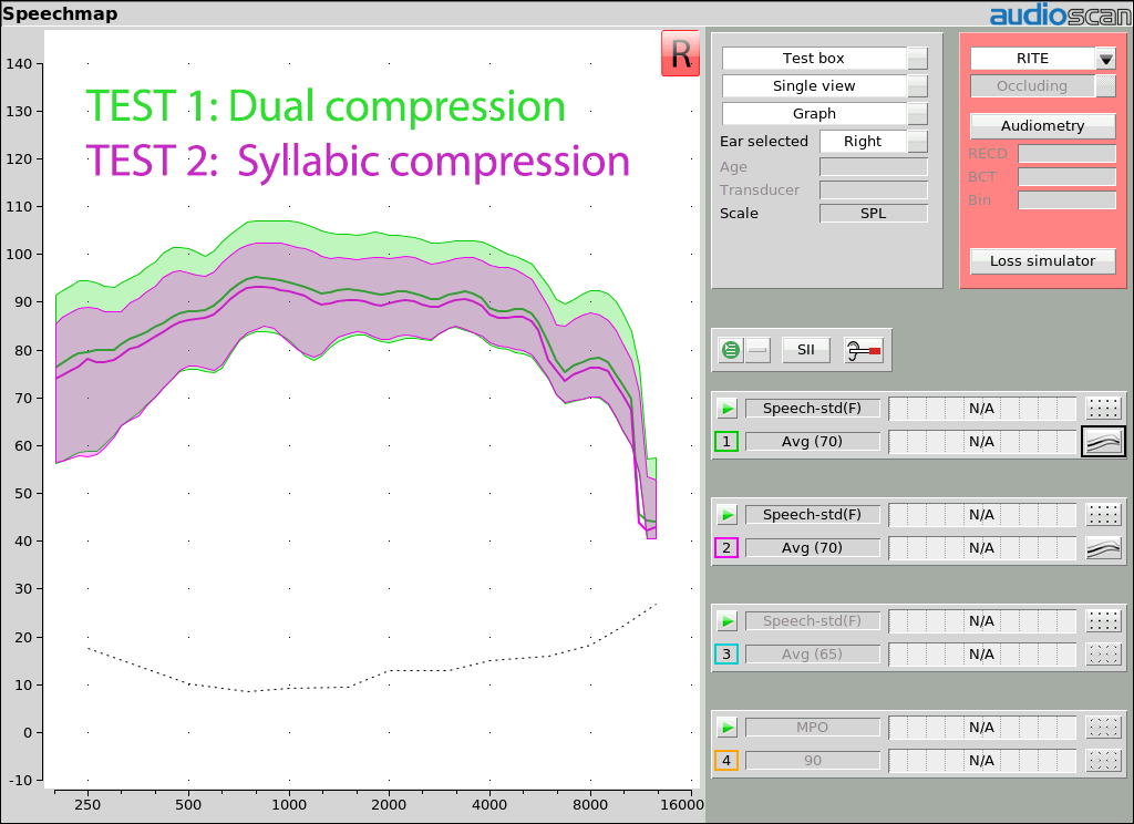
Example 1: Syllabic compression’s reduces the width of the speech region.
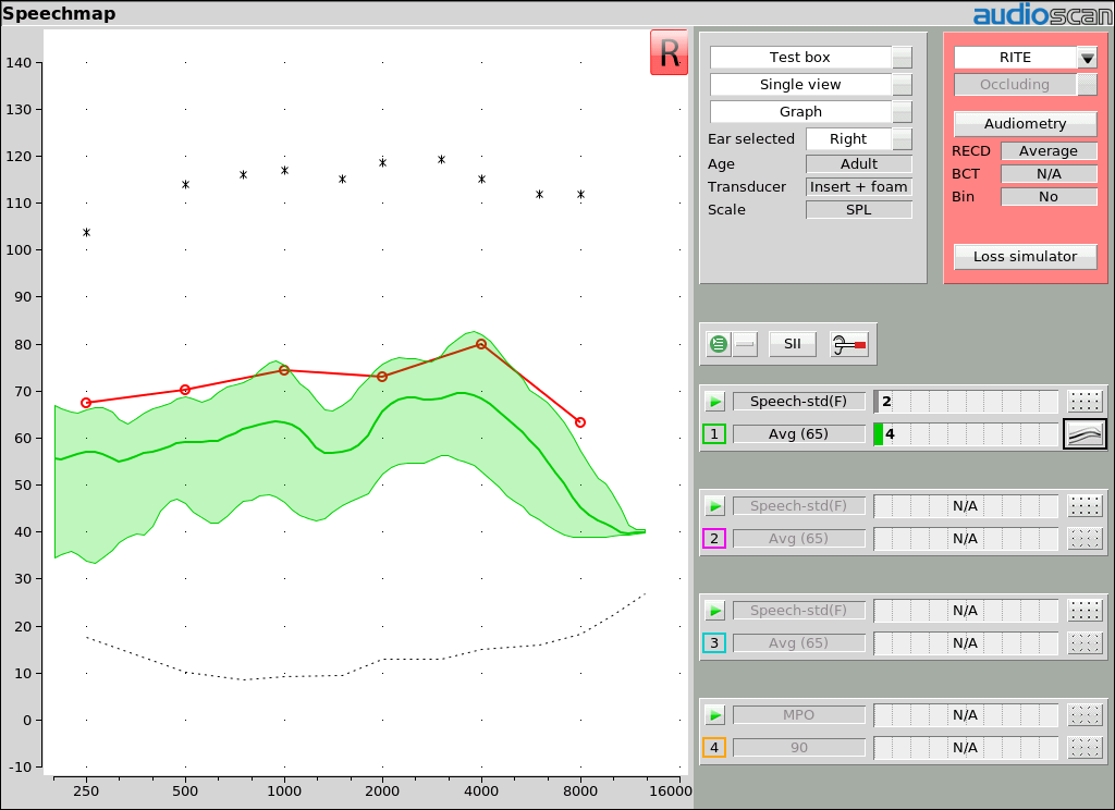
Example 2: Speech peaks at threshold, SII = 4. Speech is detectable but not understood.
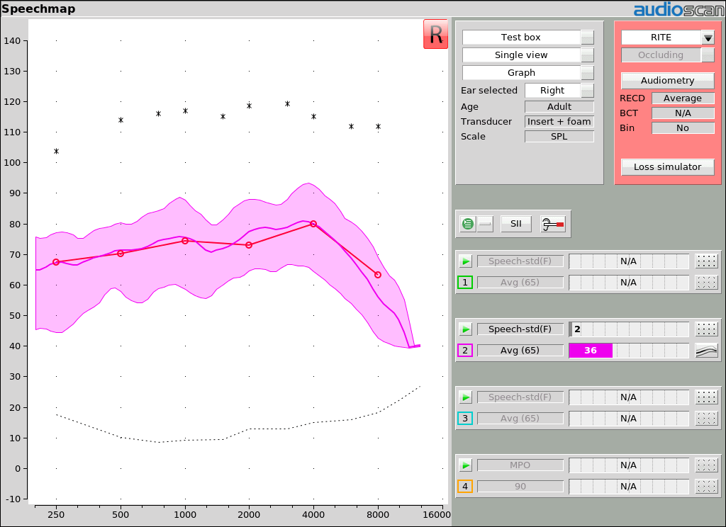
Example 3: LTASS at threshold gives an SII of 30-40, indicating 60-80% correct on the CST test (theoretical for normals).
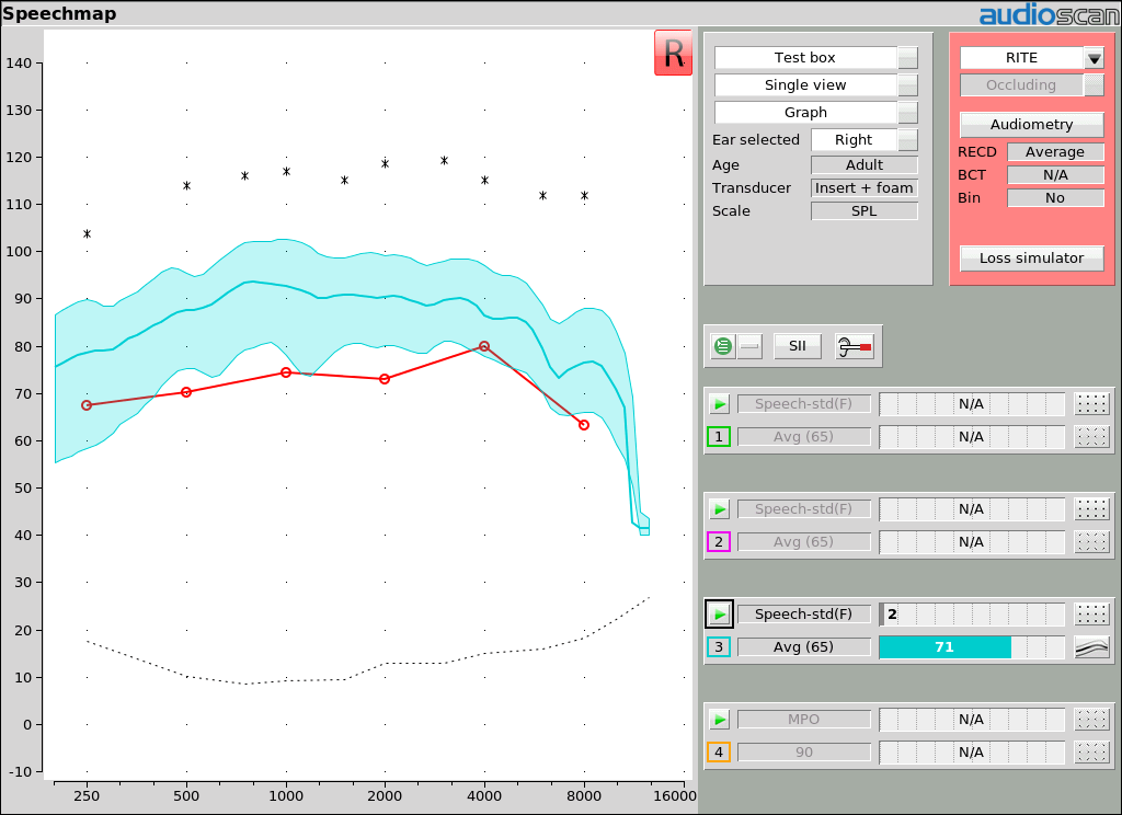
Example 4: Speech region all above threshold will result in SII above 70 which predicts a 100% score on the CST. Providing additional gain for speech at this level (65 dB SPL) will not increase understanding for this sort of speech material.